TX00CQ31 – Digital Signal Processing
Study 4: Poles and Zeros
|
Read these instructions first!
|
Number |
Questions |
Write your answer in this column |
Hints |
|
Q1 |
System
difference equation is y[n]
– 0,4y[n-1] = x[n] – 0,5x[n-1] + 0,06x[n-2] Describe
the system parameters such that you can use them in Octave/Matlab |
Commands: n = -10:100; x = n >= 0; aa = [1,-0.4,0]; % X(z) = 1 - 0.5 * z^-1 + 0.06 * z^-2 bb = [1,-0.5,0.06]; % Y(z) = 1 - 0.4 * z^-1 + 0 * z^-2 y = filter(bb,aa,x); |
see
lab 2, how you put those system
parameters to the filter command |
|
Q2 |
Draw Argand’s diagram (=zero-pole plot) and determine if
the system is stable or not. |
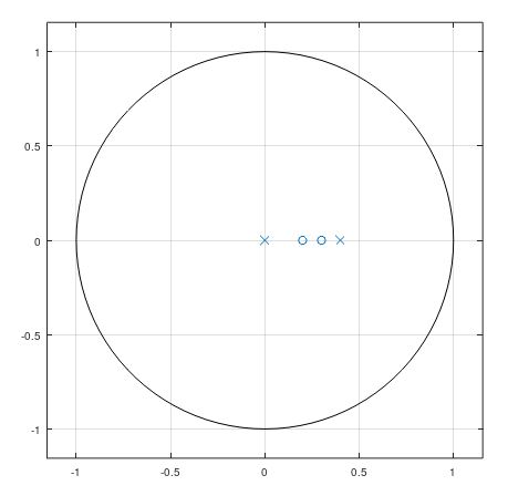 Is
the system stable? Yes, because all the poles reside inside the unit circle. |
zplane() |
|
Q3 |
Calculate
the zeros and poles of the system. |
Commands: zz = roots(bb) zz = 0.3000 0.2000 pp = roots(aa) pp = 0.4000 0 |
roots() |
|
Q4 |
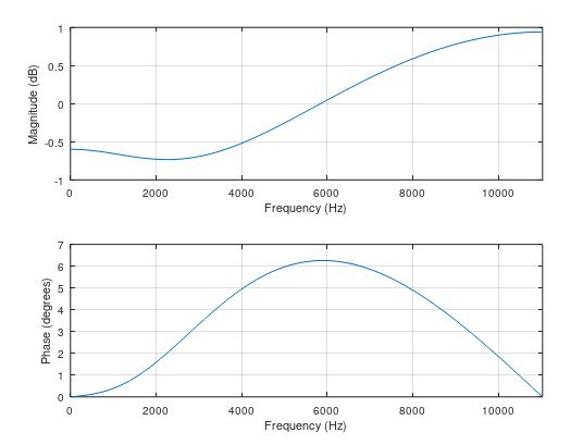
Generate
Frequency Response using sampling rate of 22050 s-1 |
 |
freqz() |
|
Q5 |
Determine
if the system is IIR or FIR by testing it with impulse function. |
IIR/FIR, why? FIR, because by time the output value tends to return to zero (after 822 samples). |
filter() |
|
Q6 |
A second
degree system has the following zero-pole plot.
Determine
the zero and pole coordinates. |
Zeros
are… Poles
are… and
that can be verified from this picture… 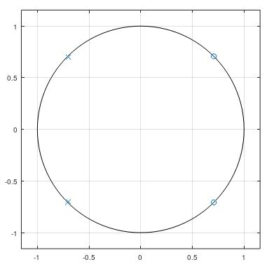 |
[ ; ] |
|
Q7 |
Determine
the corresponding system parameters (in Octave/Matlab
form). |
Commands: aan = poly(ppn) aan =
1.0000 1.4000 0.9800 bbn = poly(zzn) bbn =
1.0000 -1.4142 1.0000 The difference equation: y[n]+ 1,4y[n-1] + 0,98y[n-2] = x[n] -1.412x[n-1] + x[n-2] |
poly |
|
Q8 |
Determine
the maximum gain and rescale the system such that it has unity gain passband.
Generate
Frequency Response to verify it. |
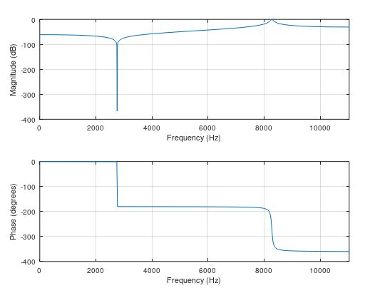 |
freqz |
|
Q9 |
Just for fun, filter a white noise audio sample with the filter and describe how your system changes the signal. Use a reasonable sampling rate (8000, 11025, 22050, 44100) in your test. |
Commands: n = -10:1000; x = n >= 0; for i = 1:length(n) q(i) = rand(); end noisy_signal = x .* q; noise_output = filter(bbns,aan,noisy_signal) 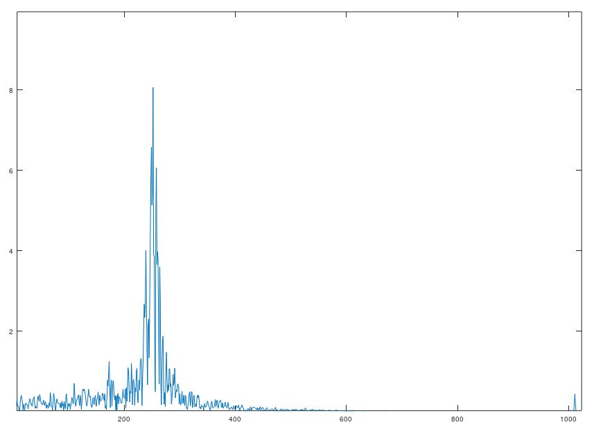 |
White noise: try
randn() |