TX00CQ31 –Digital Signal Processing
Study 2: Time
Domain
|
Read the lab instructions first!
|
Number |
Questions |
Write your answer in this column |
Hints |
|
1 |
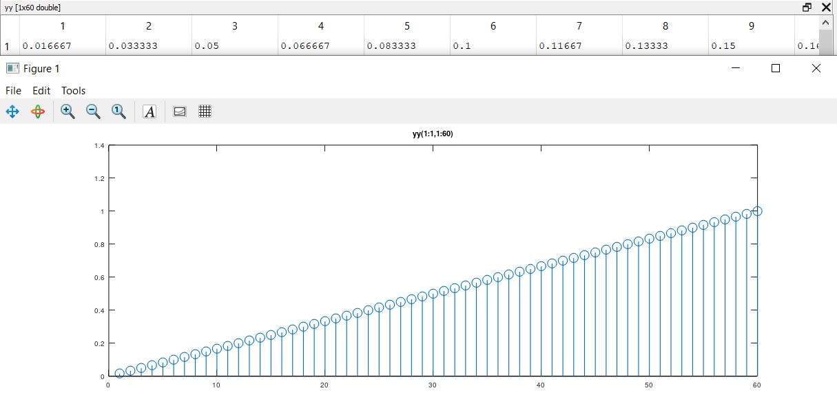
Generate an impulse response function of a running average filter with length 60. |
Commands: ss = 60; oo = ones(1, ss); run_ave_filter = oo / ss; |
ones |
|
2 |
Filter-function
is an implementation of a linear, time-invariant system in Octave. It can be
used to produce output of a FIR-system the following way: |
Commands: yy = filter(run_ave_filter, 1, oo); |
filter |
|
3 |
An easy
way to produce a delayed signal in Octave, is to use the filter-function the
following way: |
Commands: delayed_yy = filter([zeros(1,60),1],1,oo); |
filter |
|
|
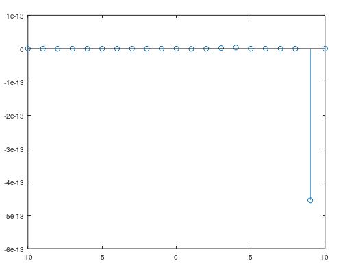
Use appropriate test vectors to check
if the system y[n] = x[n]*en is
|
Commands to verify linearity: n = -10:10; a = rand(1, 1); b = rand(1, 1); x1 = rand(1, length(n)); x2 = rand(1, length(n)); y1 = (a * x1 + b * x2) .* exp(n); y2 = a * (x1 .* exp(n)) + b * (x2 .* exp(n));
y[n] is linear, because the linearity equations provide the same values for both sides (y1-y2 is zero) and superposition is only possible in linear systems. |
Linearity: use two, random test vectors x1
and x2, and two random numbers to see if |
|
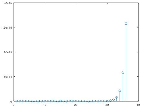
4 b |
|
Commands to verify time shift invariant: n = 0:30; x = n >= 0; y = x .* exp(n); y1_delayed = [zeros(1,5), y]; N = 0:35; x_shifted(N >= k) = 1; y2_delayed = x_shifted .* exp(N); y_difference = y2_delayed - y1_delayed;
The larger the n, the larger the difference of D{F{x}} and F{D{x}}, which implies that the system is time variant. |
Time-shift
invariance:
use step function to see if time shifted input results in an output equal to
time shifted original output |
|
4 c |
|
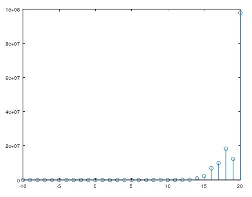
Commands to verify causality: n = -10:20; u = n >= 0; for i = 1:length(n) q(i) = rand(); end x = u .* q; y = x .* exp(n); stem(n, y);
The system is causal, because on there is no non-zero output before input. |
Causality: use a random signal, which
starts at origin as your test signal to see if the system gives non-zero
output before input |
|
4 d |
|
Commands to verify stability: n = -30:30; x = n >= 0; syms x L = limit(x .* exp(x),x,inf) Output: L = (sym) oo
As n approaches infinity, the output approaches infinity as well. Thus the system is not stable. |
Stable: test, if the step response
converges |
|
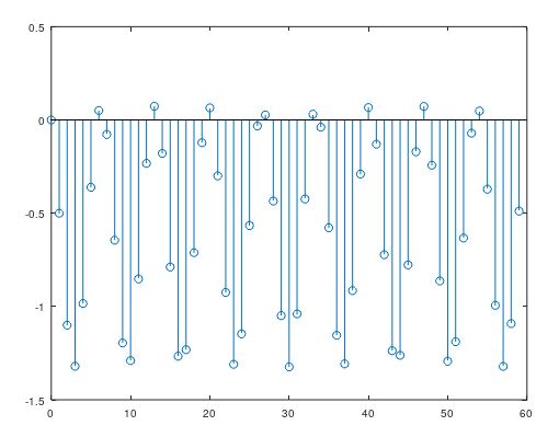
5 |
System
difference equation is: |
Commands: n = 0:59; x = n >= 0; y = filter([0,-0.5],[1,-1.2,1], x);
It is an IIR system, because it never returns to zero. |
filter |
|
6 |
Write an
m-function, which returns discrete delta function values for a given index
vector. |
Commands: function m = delta_func(n) m = (n == 0); |
|