TX00CQ31 – Digital Signal Processing

Study 1: Basics

Read the lab instructions first!

Write your answer in this column
oo = ones(1,8); % variable name = oo
n = -9:20; % Colon operator can create vectors, subscript arrays, and specify for iterations
u = n >= 0; 
d = n == 0;
x1 = (n-2 == 0) + (n == 0) - 2 * (n-1 == 0);
x2 = (n+2 >= 0) - (n-2 >= 0);
x3 = cos(0.1*pi*n);
x4 = cos(2*pi*n);
t = (1/2000)*n;
s = 0.5*cos(2*pi*960*t);
x = ((n >= 0) .* s)+2*(n-4 == 0); (’.*’ elementwise multiplication). Now you can use the original time-index vector
 (use the original index-vector from the Question 1 as x-coordinates to the stem plot)

   time_vector = linspace(0, 2, 8000*2);
   tau = 0.96;
   decay = 025 * exp(-time_vector/tau);
   sine_wave = decay .* cos(2*pi*2*960*time_vector);
   noise = 0.005 * randn(size(time_vector));
   stem(audio, time_vector);
  
sound(audio, 8000);Sounds like an artificial background noise that would have been added to an old black and white documentary to give the incoming artillery missile some sound.

Number	Questions	Write your answer in this column
0	This is an example row, showing how to produce a vector of ones	oo = ones(1,8); % variable name = oo
0	Create an index-vector from -9 to 20	n = -9:20; % Colon operator can create vectors, subscript arrays, and specify for iterations
1	Use the previous vector to generate a unit step function	u = n >= 0; (Notice that the vector is one possible argument to the arithmetic comparison operator)
2	Create a unit impulse function	d = n == 0;
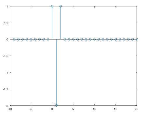
3	Create a data sequence: (see exercise 1.1 a) x1[n] = d[n-2] + d[n] - 2d[n-1]	x1 = (n-2 == 0) + (n == 0) - 2 * (n-1 == 0);
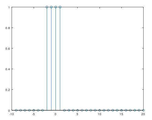
4	Create a data sequence: (see exercise 1.1 b) x2[n] = u[n+2] - u[n-2]	x2 = (n+2 >= 0) - (n-2 >= 0);
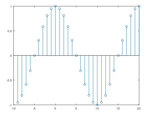
5	Create a data sequence: (see exercise 1.1 c) x3[n] = cos(0,1 pi n)	x3 = cos(0.1pin); (Notice that 0.1p is the digital frequency (rads/sample))
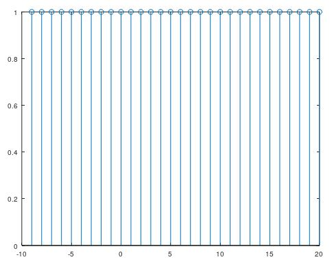
6	Create a data sequence: (see exercise 1.1 d) x4[n] = cos(2 pi n)	x4 = cos(2pin);
7	Create a time vector from the (sample) index-vector from Question 0 when the sampling rate is 2000 Hz (s^-1)	t = (1/2000)*n; (To convert from (sample) index vector to time vector you need to multiply index vector with the time between samples. From the lecture1 slides (slide 19) you find that to be T=1/fs where fs is the sampling rate (in Hz))
8	Use your time vector of Question 7 to produce the sampled data vector of a sine wave with Amplitude of 0.5 Signal frequency of 960 Hz	s = 0.5cos(2pi960t); (Now when you have time values, you can use the normal analog frequency (Hz). To convert that to rads/s (suitable for the cos-function) you need to multiply is with 2p, e.g. 2pif, where f is in Hz.)
9	Create a data sequence: x[n] = u[n]s[n] + 2d[n-4] where, u[n] = unit step function s[n] = previous, sampled sine d[n] = delta function	x = ((n >= 0) .* s)+2(n-4 == 0); (’.’ elementwise multiplication). Now you can use the original time-index vector
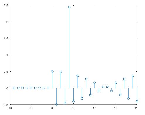
10	Stem-plot the previous data vector	(use the original index-vector from the Question 1 as x-coordinates to the stem plot)
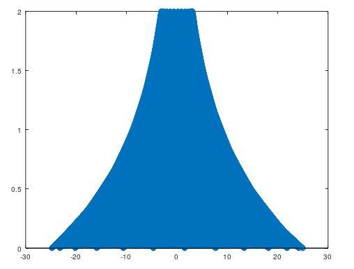
11	Generate a sound sample which consists of 8000 s^-1 sampling rate 2 second long sample Decaying sine wave Maximum amplitude 0.25 Amplitude decays exponentially with time constant of 960 ms Signal frequency (2*960) Hz Random noise, standard deviation of 0.005	time_vector = linspace(0, 2, 80002); tau = 0.96; decay = 025 exp(-time_vector/tau); sine_wave = decay .* cos(2pi2960time_vector); noise = 0.005 * randn(size(time_vector)); stem(audio, time_vector);
12	Listen to your sound sample	sound(audio, 8000); Sounds like an artificial background noise that would have been added to an old black and white documentary to give the incoming artillery missile some sound.